This vignette covers FUNDEB (Fundo de Manutencao e Desenvolvimento da Educacao Basica), the main funding mechanism for basic education in Brazil. educabR provides two functions to access FUNDEB data: resource distribution and enrollment counts.
Overview
FUNDEB redistributes tax revenues to fund basic education across states and municipalities. The data is split into two components:
| Function | Source | Description |
|---|---|---|
get_fundeb_distribution() |
STN (National Treasury) | Monthly transfers by state/municipality and funding source |
get_fundeb_enrollment() |
FNDE (OData API) | Enrollment counts used for funding calculation |
FUNDEB Distribution
Resource distribution data shows how much money was transferred to each state and municipality, broken down by funding source and month.
Funding sources
FUNDEB aggregates revenue from multiple tax sources:
| Source | Description |
|---|---|
| FPE | State Participation Fund |
| FPM | Municipal Participation Fund |
| IPI | Tax on Industrialized Products |
| ITR | Rural Property Tax |
| VAAF | Fiscal Value-Added (state portion) |
| VAAT | Total Value-Added |
| VAAR | FUNDEB Complementation |
| ICMS | State Sales Tax |
| IPVA | Vehicle Tax |
| ITCMD | Inheritance and Donation Tax |
Downloading distribution data
# All distribution data for 2023
dist_2023 <- get_fundeb_distribution(year = 2023)

# Filter by state
dist_sp <- get_fundeb_distribution(year = 2023, uf = "SP")

# Filter by funding source
dist_fpm <- get_fundeb_distribution(year = 2023, source = "FPM")

# Filter by destination (states or municipalities)
dist_estados <- get_fundeb_distribution(
  year        = 2023,
  destination = "estados"
)Data structure
dist <- get_fundeb_distribution(2023, uf = "SP")
glimpse(dist)
Example analysis: Monthly transfers by source
dist <- get_fundeb_distribution(2023, uf = "SP")

# Total monthly transfers by funding source
monthly <-
  dist |>
  mutate(mes = as.integer(format(as.Date(mes_ano), "%m"))) |>
  group_by(origem, mes) |>
  summarise(total = sum(valor, na.rm = TRUE), .groups = "drop")

ggplot(monthly, aes(x = factor(mes), y = total / 1e6, fill = origem)) +
  geom_col() +
  labs(
    title = "FUNDEB Transfers to Sao Paulo by source (2023)",
    x     = "Month",
    y     = "Total (millions R$)",
    fill  = "Source"
  ) +
  theme_minimal() +
  theme(legend.position = "bottom") +
  scale_y_continuous(labels = scales::number_format(big.mark = ".", decimal.mark = ",")) +
  guides(fill = guide_legend(nrow = 1))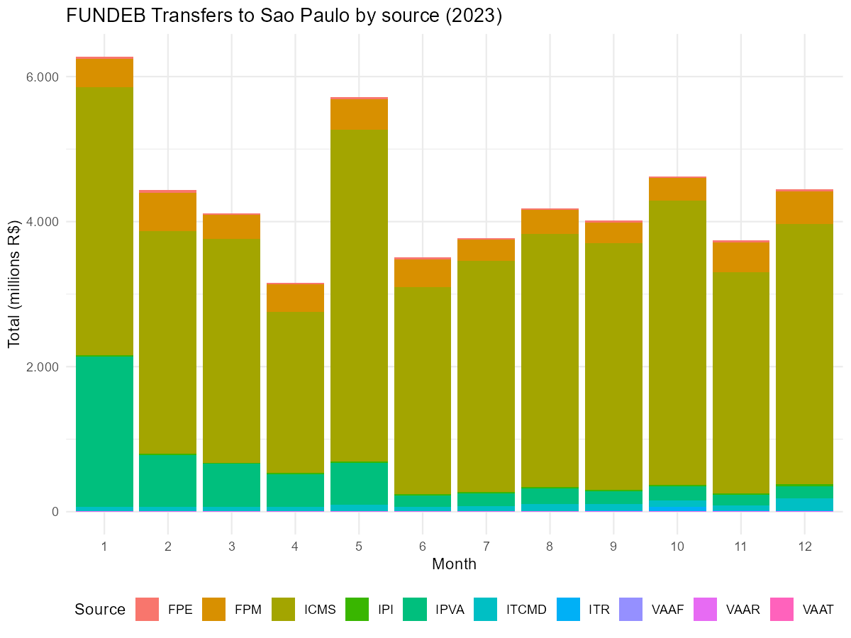
Example analysis: Comparing states
dist <- get_fundeb_distribution(2023)

# Total annual transfers by state
by_state <-
  dist |>
  group_by(uf) |>
  summarise(total = sum(valor, na.rm = TRUE), .groups = "drop") |>
  arrange(desc(total)) |>
  head(10)

ggplot(by_state, aes(x = reorder(uf, total), y = total / 1e9)) +
  geom_col(fill = "darkgreen") +
  coord_flip() +
  labs(
    title = "Top 10 States by FUNDEB Transfers (2023)",
    x     = NULL,
    y     = "Total (billions R$)"
  ) +
  theme_minimal()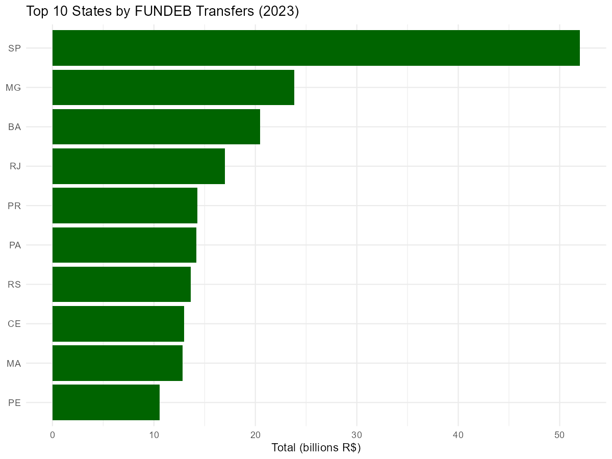
FUNDEB Enrollment
Enrollment data shows the number of students considered for FUNDEB funding calculation, broken down by municipality, education type, school network, and location.
Downloading enrollment data
# All enrollment data for 2018
mat_2018 <- get_fundeb_enrollment(year = 2018)

# Filter by state (filtered locally from cached complete dataset)
mat_sp <- get_fundeb_enrollment(year = 2018, uf = "SP")

# Limited rows for exploration
mat_sample <- get_fundeb_enrollment(year = 2018, n_max = 5000)
Available years
Data is available for 2017-2018. Data is fetched from the FNDE OData API with automatic pagination.
Data structure
The enrollment data contains these columns:
| Column | Description |
|---|---|
ano_censo |
Census year |
uf |
State code |
municipio |
Municipality name |
tipo_rede_educacao |
Education network type |
descricao_tipo_educacao |
Education type description |
descricao_tipo_ensino |
Teaching type description |
descricao_tipo_turma |
Class type description |
descricao_tipo_carga_horaria |
Class hours type |
descricao_tipo_localizacao |
Location type (urban/rural) |
qtd_matricula |
Number of enrollments |
mat <- get_fundeb_enrollment(2018, uf = "RJ")
glimpse(mat)
Example analysis: Enrollment by education type
mat <- get_fundeb_enrollment(2018, uf = "SP")

# Total enrollment by education type
by_type <-
  mat |>
  group_by(descricao_tipo_educacao) |>
  summarise(total = sum(qtd_matricula, na.rm = TRUE), .groups = "drop") |>
  arrange(desc(total))

ggplot(by_type, aes(x = reorder(descricao_tipo_educacao, total), y = total / 1e3)) +
  geom_col(fill = "coral", width = .5) +
  coord_flip() +
  labs(
    title = "FUNDEB Enrollment by Education Type - SP (2018)",
    x     = NULL,
    y     = "Enrollments (thousands)"
  ) +
  theme_minimal() +
  scale_y_continuous(labels = scales::number_format(big.mark = ".", decimal.mark = ","))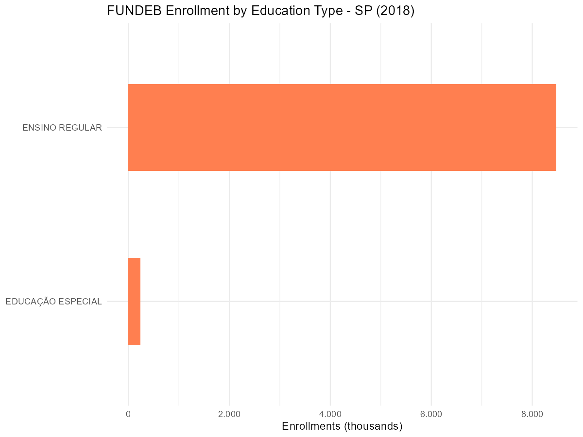
Example analysis: Urban vs rural enrollment
mat <- get_fundeb_enrollment(2018)

# Compare urban vs rural
by_location <-
  mat |>
  mutate(
    location = case_when(
      descricao_tipo_localizacao == "URBANA"     ~ "Urban",
      descricao_tipo_localizacao == "RURAL"      ~ "Rural",
      descricao_tipo_localizacao == "QUILOMBOLA" ~ "Quilombola",
      descricao_tipo_localizacao == "IND\u00cdGENA" ~ "Indigenous",
      .default = descricao_tipo_localizacao
    )
  ) |>
  group_by(uf, location) |>
  summarise(total = sum(qtd_matricula, na.rm = TRUE), .groups = "drop")

ggplot(by_location, aes(x = uf, y = total / 1e3, fill = location)) +
  geom_col(position = "dodge") +
  labs(
    title = "FUNDEB Enrollment: Urban vs Rural by State (2018)",
    x     = "State",
    y     = "Enrollments (thousands)",
    fill  = "Location"
  ) +
  theme_minimal() +
  theme(axis.text.x = element_text(angle = 45, hjust = 1)) +
  scale_y_continuous(labels = scales::number_format(big.mark = ".", decimal.mark = ","))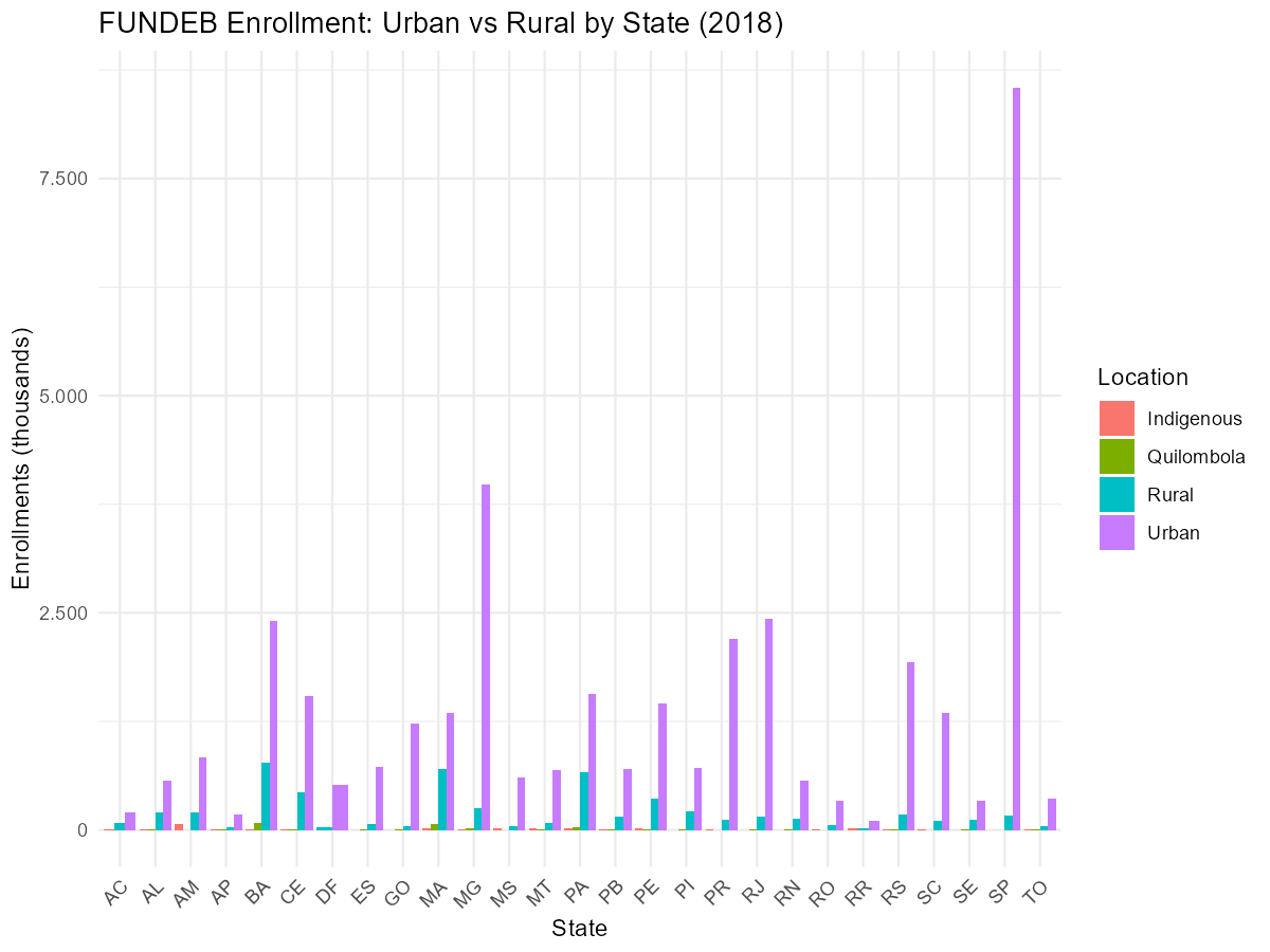
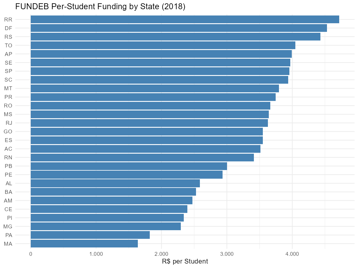
Combining distribution and enrollment
You can combine both datasets to analyze per-student funding across states.
# Total transfers by state
dist <- get_fundeb_distribution(2018)
transfers <-
  dist |>
  group_by(uf) |>
  summarise(total_transfer = sum(valor, na.rm = TRUE), .groups = "drop")

# Total enrollment by state
mat <- get_fundeb_enrollment(2018)
enrollment <-
  mat |>
  group_by(uf) |>
  summarise(total_students = sum(qtd_matricula, na.rm = TRUE), .groups = "drop")

# Per-student funding
funding <-
  inner_join(transfers, enrollment, by = "uf") |>
  mutate(per_student = total_transfer / total_students) |>
  arrange(desc(per_student))

ggplot(funding, aes(x = reorder(uf, per_student), y = per_student)) +
  geom_col(fill = "steelblue") +
  coord_flip() +
  labs(
    title = "FUNDEB Per-Student Funding by State (2018)",
    x     = NULL,
    y     = "R$ per Student"
  ) +
  theme_minimal() +
  scale_y_continuous(labels = scales::number_format(big.mark = ".", decimal.mark = ","))