Mapping education indicators with geobr
Source:vignettes/mapping-education-with-geobr.Rmd
mapping-education-with-geobr.RmdThis vignette shows how to combine educabR with geobr to create choropleth maps of education indicators across Brazilian municipalities and states.
IDEB by state
The simplest map uses state-level data. We download IDEB scores and join them with state geometries from geobr.
ideb_uf <-
  get_ideb(level = "estado", stage = "anos_iniciais", metric = "indicador", year = 2023) |>
  filter(rede == "Total", indicador == "IDEB")

states <- read_state(year = 2020, showProgress = FALSE)

states |>
  left_join(ideb_uf, by = c("abbrev_state" = "uf_sigla")) |>
  ggplot() +
  geom_sf(aes(fill = valor), color = "white", linewidth = .2) +
  scale_fill_distiller(palette = "YlGn", direction = 1, name = "IDEB") +
  labs(title = "IDEB 2023 — Early elementary by state") +
  theme_void()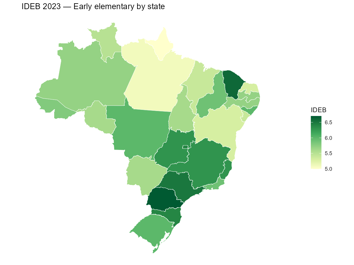
IDEB by municipality
Municipality-level maps reveal within-state inequality that state
averages hide. The municipio_codigo column in educabR uses
the 7-digit IBGE code, which matches code_muni in
geobr.
ideb_muni <- get_ideb(
  level  = "municipio",
  stage  = "anos_iniciais",
  metric = "indicador",
  year   = 2023
)

# Keep only public schools and the IDEB indicator
ideb_muni <-
  ideb_muni |>
  filter(rede == "P\u00fablica", indicador == "IDEB")

municipalities <- read_municipality(year = 2020, showProgress = FALSE)
municipalities |>
  mutate(code_muni = as.character(code_muni)) |>
  left_join(ideb_muni, by = c("code_muni" = "municipio_codigo")) |>
  ggplot() +
  geom_sf(aes(fill = valor), color = NA) +
  scale_fill_distiller(palette = "YlGn", direction = 1, name = "IDEB") +
  labs(title = "IDEB 2023 — Early elementary by municipality (public schools)") +
  theme_void()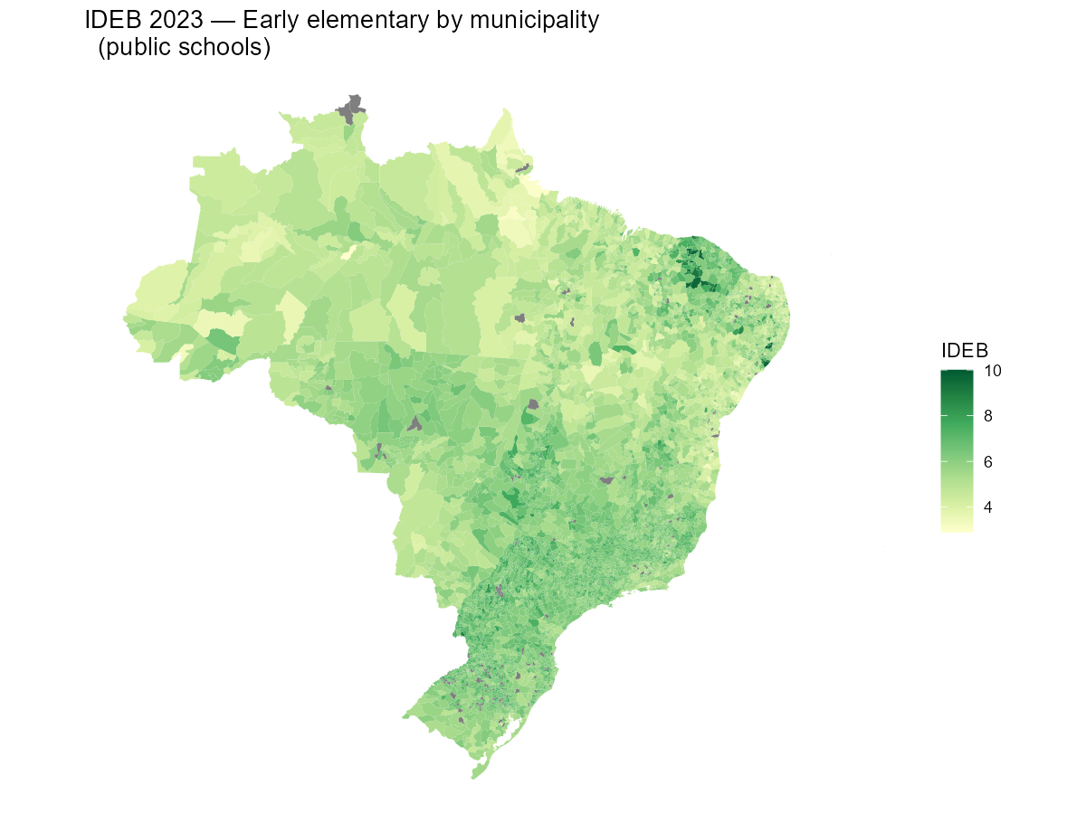
Zooming into a single state
For a closer look, filter both datasets to a single state. Here we map IDEB across municipalities in Minas Gerais.
ideb_mg <-
  ideb_muni |>
  filter(uf_sigla == "MG")

munis_mg <- read_municipality(code_muni = "MG", year = 2020, showProgress = FALSE)

munis_mg |>
  mutate(code_muni = as.character(code_muni)) |>
  left_join(ideb_mg, by = c("code_muni" = "municipio_codigo")) |>
  ggplot() +
  geom_sf(aes(fill = valor), color = "grey90", linewidth = .1) +
  scale_fill_distiller(palette = "YlGn", direction = 1, name = "IDEB") +
  labs(title = "IDEB 2023 — Early elementary in Minas Gerais") +
  theme_void()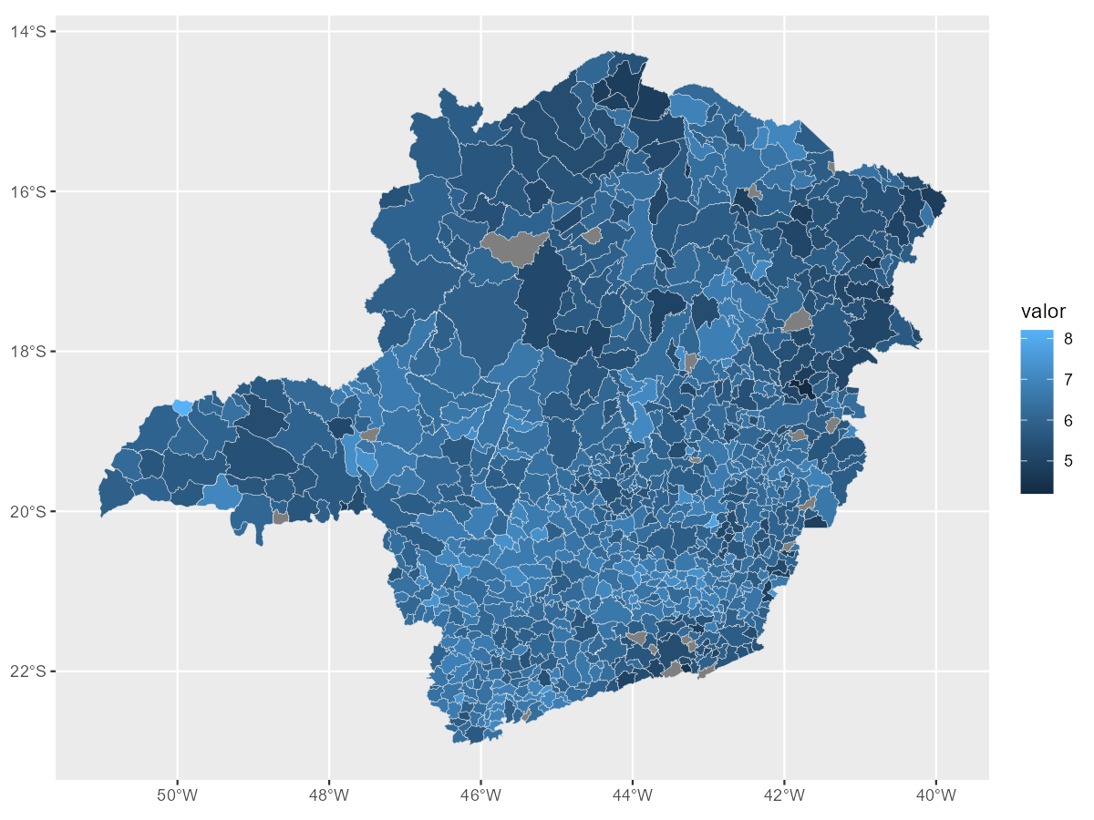
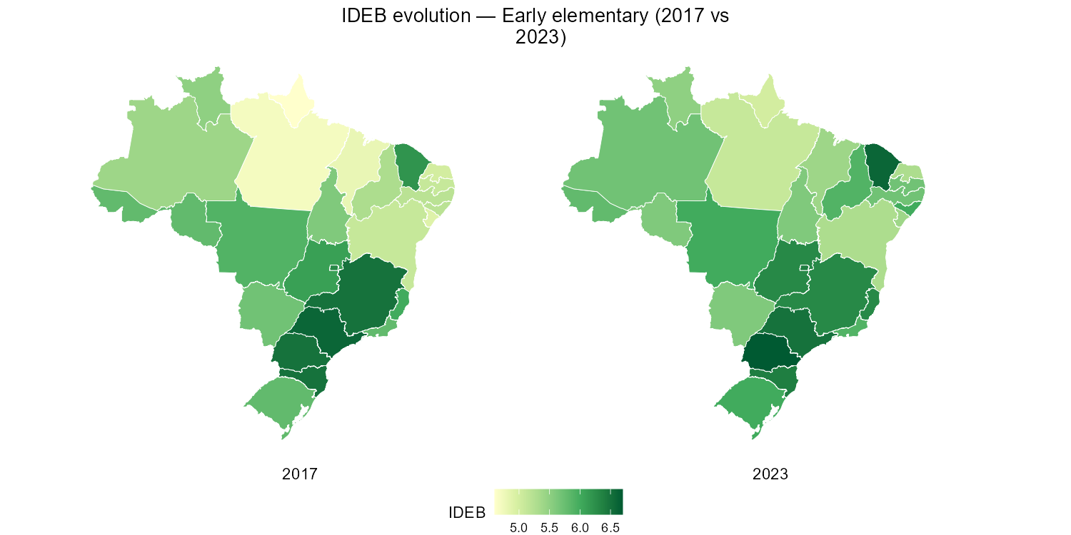
Comparing IDEB editions over time
Side-by-side maps make it easy to visualize regional progress. We download two editions and use facets.
ideb_time <-
  get_ideb(
    level  = "estado",
    stage  = "anos_iniciais",
    metric = "indicador",
    year   = c(2017, 2023)
  ) |>
  filter(rede == "Total", indicador == "IDEB")

states |>
  left_join(ideb_time, by = c("abbrev_state" = "uf_sigla")) |>
  ggplot() +
  geom_sf(aes(fill = valor), color = "white", linewidth = .2) +
  scale_fill_distiller(palette = "YlGn", direction = 1, name = "IDEB") +
  facet_wrap(~ano, strip.position = "bottom") +
  labs(title = "IDEB evolution — Early elementary (2017 vs 2023)") +
  theme_void() +
  theme(
    legend.position = "bottom",
    plot.title = element_text(hjust = 0.5),
    strip.text = element_text(size = 11, margin = margin(t = 5))
  )
Next steps
- Swap
"anos_iniciais"for"anos_finais"or"ensino_medio"to map other stages. - Use
metric = "nota"to map SAEB proficiency scores instead of the composite IDEB. - Combine with other educabR datasets (ENEM, School Census) using the same municipality codes.
- See the geobr documentation for additional geographic layers (regions, micro/mesoregions, etc.).